The ECG leads: Electrodes, limb leads, chest (precordial) leads and the 12-Lead ECG
The ECG leads
- The electrophysiological basis of the ECG leads
- The 12-lead ECG
- The ECG paper
- Derivation of the ECG leads
- Anatomical planes and ECG leads
- Principles of the limb leads
- ECG Leads I, II and III (Willem Einthoven’s original leads)
- ECG lead aVR, aVF and aVL (Goldberger’s leads)
- Chest leads (precordial leads)
- Presentation of ECG leads
- Additional (supplementary) ECG leads
- Alternative ECG lead systems
- Mason-Likar ECG lead system
- Reduced ECG lead systems
Before discussing the ECG leads and various lead systems, we need to clarify the difference between ECG leads and ECG electrodes. An electrode is a conductive pad that is attached to the skin and enables the recording of electrical currents. An ECG lead is a graphical description of the electrical activity of the heart and it is created by analyzing several electrodes. In other words, each ECG lead is computed by analyzing the electrical currents detected by several electrodes. The standard ECG – which is referred to as a 12-lead ECG since it includes 12 leads – is obtained using 10 electrodes. These 12 leads consist of two sets of ECG leads: limb leads and chest leads. The chest leads may also be referred to as precordial leads. This article will discuss the ECG leads in detail and no prior knowledge is required. Note that the terms unipolar leads and bipolar leads are not recommended because all ECG leads are bipolar, since they compare electrical currents in two measurement points.
The electrophysiological basis of the ECG leads
The movement of charged particles generates an electric current. In electrocardiology, these charged particles are represented by intracellular and extracellular ions, such as sodium (Na+), potassium (K+), and calcium (Ca2+). These ions flow across cell membranes, enabling depolarization and repolarization, and between cells via gap junctions, facilitating the propagation of depolarization across the cells.
Electrical potential differences arise as the electrical impulse travels through the heart. Electric potential difference is defined as a difference in electric potential between two measurement points. In electrocardiology, these measurement points are the skin electrodes. Thus, the electrical potential difference is the difference in the electrical potential detected by two (or more) electrodes.
The previous discussion outlined how depolarization and repolarization generate electrical currents. It was also explained that the electrical currents are conducted all the way to the skin, because the tissues and fluids surrounding the heart, indeed the entire human body, act as electrical conductors. By placing electrodes on the skin it is possible to detect these electrical currents. The electrocardiograph (ECG machine) compares, amplifies and filters the electrical potential differences recorded by the electrodes and presents the results as ECG leads. Each ECG lead is presented as a diagram (sometimes called a curve).
The 12-lead ECG
Numerous ECG lead systems and constellations of leads have been tested but the standard 12-lead ECG is still the most used and the most important lead system to master. The 12-lead ECG offers outstanding possibilities to diagnose abnormalities. Importantly, the vast majority of recommended ECG criteria (e.g. criteria for acute myocardial infarction) have been derived and validated using the 12-lead ECG.
The 12-lead ECG displays, as the name implies, 12 leads which are derived by means of 10 electrodes. Three of these leads are easy to understand since they are simply the result of comparing electrical potentials recorded by two electrodes; one electrode is exploring, while the other is a reference electrode. In the remaining 9 leads the exploring electrode is still just one electrode but the reference is obtained by combining two or three electrodes.
At any given instant during the cardiac cycle, all ECG leads analyze the same electrical events but from different angles. This means that ECG leads with similar angles must display similar ECG curves (diagrams). For some purposes (e.g. diagnosis of some arrhythmias) it is not always necessary to analyze all leads, as the diagnosis can often be established by examining fewer leads. On the other hand, for the purpose of diagnosing morphological changes (e.g. myocardial ischemia, ventricular hypertrophy), the ability to do so increases as the number of leads increases. The 12-lead ECG is a trade-off between sensitivity, specificity, and feasibility. Obviously, having 120 leads (which has been tested in several studies on acute myocardial infarction) would improve sensitivity for many conditions, at the expense of specificity and certainly feasibility. Subsequent chapters will clarify why multiple leads are required to diagnose many morphological changes.
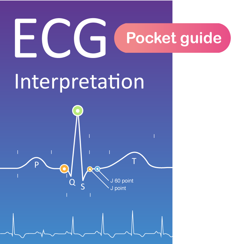
The ECG paper
The electrocardiograph presents one diagram for each lead. Voltage is presented on the vertical (Y) axis and time on the horizontal (X) axis of the diagram. The ECG paper has small boxes (thin lines) and large boxes (heavy lines). Small boxes are squares of 1 mm2 and there are 5 small boxes inside each large box. Refer to Figure 15.
With normal gain (calibration) 10 mm on the vertical axis corresponds to 1 mV. Thus, 1 mm corresponds to 0.1 mV. The amplitude (height) of a wave/deflection is measured from the maximum of the wave/deflection to the baseline (also called the isoelectric line).
The ECG paper speed is generally 25 mm/s or 50 mm/s (10 mm/s may be used for longer recordings). All modern ECG machines can switch between these paper speeds and the choice of speed does not affect any aspect of ECG interpretation (although the waves are better delineated using 50 mm/s). Anyone aiming to become proficient in ECG interpretation must master any paper speed. The figure below (Figure 15) shows the differences between 50 mm/s and 25 mm/s. This figure should be studied carefully and attention should be paid to differences on the X-axis (there are no differences with respect to the Y-axis). Both 25 mm/s and 50 mm/s will be used to present the ECG tracings in this course.

As evident from Figure 15:
- 1 small box (1 mm) is 0.02 seconds (20 milliseconds) at 50 mm/s.
- 1 small box ( 1mm) is 0.04 seconds (40 milliseconds) at 25 mm/s.
- 1 large box (5 mm) is 0.1 seconds (100 milliseconds) at 50 mm/s.
- 1 large box (5 mm) is 0.2 seconds (200 milliseconds) at 25 mm/s.
The reader should know these differences as it is often necessary to manually measure the time duration of various waves and intervals on the ECG.
Derivation of the ECG leads
Every lead represents differences in electrical potentials measured in two points in space. The simplest leads are composed using only two electrodes. The electrocardiograph defines one electrode as an exploring (positive) and the other as a reference (negative) electrode. In most leads, however, the reference is composed of a combination of two or three electrodes. Regardless of how the exploring electrode and the reference are set up, the vectors have the same impact on the ECG curve. A vector heading towards the exploring electrode yields a positive wave/deflection and vice versa. Please refer to Figure 16.

Anatomical planes and ECG leads
The electrical activity of the heart can be observed from the horizontal plane and the frontal plane. The ability of a lead to detect vectors in a certain plane depends on how the lead is angled in relation to the plane, which in turn depends on the placement of the exploring lead and the reference point.
For pedagogical purposes, consider a lead with one electrode placed on the head and the other electrode placed on the left foot. The angle of this lead would be vertical, from the head to the foot. This lead is angled in the frontal plane and it will primarily detect vectors traveling in that plane. Refer to Figure 17 panel A. Now consider a lead with an electrode placed on the sternum and the other electrode placed on the back (on the same level). This lead will be angled from the back to the anterior chest wall, which is the horizontal plane. This lead will primarily record vectors traveling in that plane. A schematic illustration is provided in Figure 15. Refer to Figure 17 panel B.
Log in to view image, video, quiz, text

The limb leads, of which there are six (I, II, III, aVF, aVR and aVL), have the exploring electrode and the reference point placed in the frontal plane. These leads are therefore excellent for detecting vectors traveling in the frontal plane. The chest (precordial) leads (V1, V2, V3, V4, V5 and V6) have the exploring electrodes located anteriorly on the chest wall and the reference point located inside the chest. Hence, the chest leads are excellent for detecting vectors traveling in the horizontal plane.
As noted previously only three leads, namely leads I, II and III (which are Willem Einthoven’s original leads) are derived by using only two electrodes. The remaining nine leads use a reference which is composed of the average of either two or three electrodes. This will be clarified shortly.
Log in to view image, video, quiz, text
Principles of the limb leads
Leads I, II, III, aVF, aVL and aVR are all derived using three electrodes, which are placed on the right arm, the left arm and the left leg. Given the electrode placements, in relation to the heart, these leads primarily detect electrical activity in the frontal plane. Figure 18 shows how the electrodes are connected in order to obtain these six leads.
To explain the derivation of the limb leads, lead I and lead aVF will be used as examples.
Considering lead I the electrode on the right arm serves as the reference, whereas the electrode on the left arm serves as the exploring electrode. This means that a vector moving from right to left should yield a positive deflection in lead I. Note that Lead I defines 0° in the frontal plane (Figure 18, the coordinate system in the upper panel). This also means that lead I “views” the heart from an angle of 0°. In clinical practice, it is typically expressed as if lead I “views the lateral wall of the left ventricle”. The same principles apply to lead II and lead III.
In lead aVF the electrode on the left leg serves as the exploring electrode and the reference is composed by computing the average of the arm electrodes. The average of the arm electrodes yields a reference directly north of the left leg electrode. Thus, any vector moving downwards in the chest should yield a positive wave in lead aVF. The angle by which lead aVF views the heart’s electrical activity is 90° (Figure 18). In clinical practice, it is typically expressed as if lead aVF “views the inferior wall of the left ventricle”. The same principles apply to lead aVR and lead aVL.
Lead II, aVF and III are called inferior limb leads because they primarily observe the inferior wall of the left ventricle (Figure 18, coordinate system in upper panel). Lead aVL, I and –aVR are called lateral limb leads, because they primarily observe the lateral wall of the left ventricle. Note that lead aVR differs from lead –aVR (discussed below).
All six limb leads are presented in a coordinate system, which the right-hand side of Figure 18 (panel A) shows. There is a 30° distance between each lead, except for the gap between lead I and lead II. To eliminate this gap, lead aVR can be inverted into lead –aVR. It turns out that this is meaningful, as it facilitates ECG interpretation (e.g. interpretation of ischemia and electrical axis). Whether lead aVR or –aVR is presented depends on national traditions. In the US lead, aVR is used more frequently than –aVR. However, all modern ECG machines are capable of presenting both aVR and –aVR, and it is recommended that –aVR be used since it facilitates ECG interpretation. In any case, the clinician can easily switch between aVR and –aVR without adjusting the ECG machine; this is done simply by turning the ECG curve upside-down.
ECG Leads I, II and III (Willem Einthoven’s original leads)
Leads I, II and III compare electrical potential differences between two electrodes. Lead I compare the electrode on the left arm with the electrode on the right arm, of which the former is the exploring electrode. It is said that lead I observe the heart “from the left” because its exploring electrode is placed on the left (at an angle of 0°, see Figure 18). Lead II compares the left leg with the right arm, with the leg electrode being the exploring electrode. Therefore, lead II observes the heart from an angle of 60°. Lead III compares the left leg with the left arm, with the leg electrode being the exploring one. Lead III observes the heart from an angle of 120° (Figure 18).
Leads I, II and III are the original leads constructed by Wilhelm Einthoven. The spatial organization of these leads forms a triangle in the chest (Einthoven’s triangle) which is presented in Figure 18, panel B.
According to Kirchhoff’s law, the sum of all currents in a closed circuit must be zero. Since Einthoven’s triangle can be viewed as a circuit, the same rule should apply to it. Thus emerges Einthoven’s law:

This law implies that the sum of the potentials in lead I and lead III equals the potentials in lead II. In clinical electrocardiography, this means that the amplitude of, for example, the R-wave in lead II is equal to the sum of the R-wave amplitudes in lead I and III. It follows that we need only know the information in two leads in order to calculate the exact appearance of the remaining lead. Hence, these three leads carry two pieces of information, observed from three angles.
ECG lead aVR, aVF and aVL (Goldberger’s leads)
These leads were originally constructed by Goldberger. In these leads the exploring electrode is compared with a reference which is based on an average of the other two limb electrodes. The letter a stands for augmented, V for voltage and R is right arm, L is left arm and F is foot.
In aVR the right arm is the exploring electrode and the reference is composed by averaging the left arm and left leg. Lead aVR can be inverted into lead –aVR (which means that the exploring and reference point has switched positions), which is identical to aVR but upside-down. There are three advantages of inverting aVR into –aVR:
- –aVR fills the gap between lead I and lead II in the coordinate system.
- –aVR facilitates the calculation of the heart’s electrical axis.
- –aVR improves diagnosis of acute ischemia/infarction (inferior and lateral ischemia/infarction).
Despite these advantages lead aVR is unfortunately still used in the United States and many other countries. Luckily, all modern ECG machines can be configured to show either aVR or –aVR. We recommend the use of –aVR but for the purpose of this discussion, both leads will be presented. If only one of these leads is shown, the reader may simply turn it upside-down to get a view of the desired lead. Finally, it should be noted that very few ECG diagnoses depend on lead aVR/–aVR.
In lead aVL, the left arm electrode is exploring and the lead views the heart from –30°. In lead aVF the exploring electrode is placed on the left leg, so this lead observes the heart directly from the south.
Since Godlberger’s leads are composed of the same electrodes as Einthoven’s leads, it is not surprising that all these leads display a mathematical relation. The equations follow:
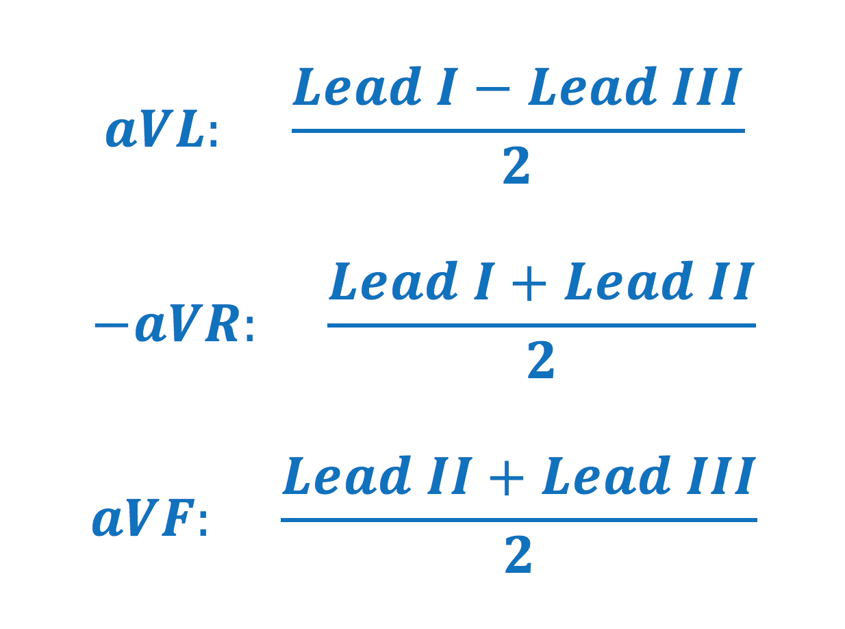
It follows that the ECG waves in lead aVF, at any given instance, is the average of the ECG deflection in leads II and III. Hence, leads aVR/–aVR, aVL and aVF can be calculated by using leads I, II and IIII and therefore these leads (aVF, aVR/–aVR, aVL) do not offer any new information, but instead new angles to view the same information.
Anatomical aspects of the limb leads
- II, aVF and III: are called inferior (diaphragmal) limb leads and they primarily observe the inferior aspect of the left ventricle.
- aVL, I and -aVR: are called lateral limb leads and they primarily observe the lateral aspect of the left ventricle.
Chest leads (precordial leads)

Frank Wilson and colleagues constructed the central terminal, later termed Wilson’s central terminal (WCT). This terminal is a theoretical reference point located approximately in the center of the thorax, or more precisely in the center or Einthoven’s triangle. WCT is computed by connecting all three limb electrodes (via electrical resistance) to one terminal. This terminal will represent the average of the electrical potentials recorded in the limb electrodes. Under ideal circumstances, the sum of these potentials is zero (Kirchoff’s law). WCT serves as the reference point for each of the six electrodes which are placed anteriorly on the chest wall. The chest leads are derived by comparing the electrical potentials in WCT to the potentials recorded by each of the electrodes placed on the chest wall. There are six electrodes on the chest wall and thus six chest leads (Figure 19). Each chest lead offers unique information that cannot be derived mathematically from other leads. Since the exploring electrode and the reference is placed in the horizontal plane, these leads primarily observe vectors moving in that plane.
Placement of chest (precordial) electrodes
- V1: fourth intercostal space, to the right of the sternum.
- V2: fourth intercostal space, to the left of the sternum.
- V3: placed diagonally between V2 and V4.
- V4: between ribs 5 and 6 in the midclavicular line.
- V5: placed on the same level as V4, but in the anterior axillary line.
- V6: placed on the same level as V4 and V5, but in the midaxillary line.
Hair on the chest wall should be shaved before the placement of electrodes. This improves the quality of the registration.
Anatomical aspects of the chest (precordial) leads
- V1-V2 (“septal leads”): primarily observes the ventricular septum, but may occasionally display ECG changes originating from the right ventricle. Note that none of the leads in the 12-lead ECG are adequate to detect vectors of the right ventricle.
- V3-V4 (“anterior leads”): observes the anterior wall of the left ventricle.
- V5-V6 (“anterolateral leads”): observes the lateral wall of the left ventricle.
Figure 20 shows the combined views of all leads in the 12-lead ECG.

Presentation of ECG leads
The ECG leads may be presented chronologically (i.e. I, II, III, aVL, aVR, aVL, V1 to V6) or according to their anatomical angles. Chronological order does not respect that leads aVL, I and -aVR all view the heart from a similar angle and placing them next to each other can improve diagnostics. The Cabrera system should be preferred. In the Cabrera system, the leads are placed in their anatomical order. The inferior limb leads (II, aVF and III) are juxtaposed, and the same goes for the lateral limb leads and the chest leads. As mentioned earlier, inverting lead aVR into –aVR improves diagnostics additionally. All modern ECG machines can display the leads according to the Cabrera system, which should always be preferred. The ECG below shows an example of the Cabrera layout with aVR inverted into –aVR. Note the clear transition between the waveforms in neighboring leads.

Additional (supplementary) ECG leads
There are conditions that may be missed when utilizing the 12-lead ECG. Fortunately, researchers have validated the use of additional leads to improve the diagnostics of such conditions. These are now discussed.
Right ventricular ischemia/infarction: ECG leads V3R, V4R, V5R and V6R
Infarction of the right ventricle is unusual but may occur if the right coronary artery is occluded proximally. None of the standard leads in the 12-lead ECG is adequate for diagnosing right ventricular infarction. However, V1 and V2 may occasionally display ECG changes indicative of ischemia located in the right ventricle. In such scenarios, it is recommended that additional leads be placed on the right side of the chest. These leads are V3R, V4R, V5R and V6R, which are placed in the same anatomical locations as their left-sided counterparts. Refer to Figure 22.

Posterolateral ischemia/infarction: ECG leads V7, V8 and V9
Considering myocardial ischemia and infarction, elevation of the ST-segment (discussed later) is an alarming finding as it implies that there is extensive ischemia. Ischemic ST-segment elevations are often accompanied by ST-segment depressions in ECG leads which view the ischemic vector from the opposite angle. Such ST-segment depressions are therefore termed reciprocal ST-segment depressions because they are mirror reflections of the ST-segment elevations. However, because the heart is rotated approximately 30° to the left in the chest (Figure 23), the basal part of the lateral left ventricular wall is positioned somewhat posteriorly (which is why it is referred to as the posterolateral wall). Electrical activity emanating from this part of the left ventricle (marked with an arrow in Figure 23) cannot be readily detected with the standard leads, but the reciprocal changes (ST-segment depressions) are commonly seen in V1–V3. In order to reveal the ST-segment elevations located posteriorly, one must attach the leads V7, V8 and V9 on the back of the patient.
Please note that right ventricular infarction and posterolateral infarction will be discussed in detail later on.

Alternative ECG lead systems

The conventional placement of electrodes can be suboptimal in some situations. Electrodes placed distally on the limbs will record too much muscle disturbance during exercise stress testing; electrodes on the chest wall may be inappropriate in case of resuscitation and echocardiographic examination etc. Efforts have been made to find alternative electrode placements, as well as reduce the number of electrodes without losing information. In general, lead systems with less than 10 electrodes can still be used to compute all leads in the standard 12-lead ECG. Such calculated ECG waveforms are very similar to the original 12-lead ECG waveforms, with some minor differences that may affect amplitudes and intervals.
As a rule of thumb, modified lead systems are fully capable of diagnosing arrhythmias but one should be cautious when using these systems to diagnose morphological conditions (e.g ischemia) that dependent on criteria for amplitudes and intervals (because the alternative electrode placement may affect these variables and cause to false positive and false negative ECG criteria). Indeed, in the setting of myocardial ischemia, one millimeter may make a life-threatening difference.
Lead systems with reduced electrodes are still used daily to detect episodes of ischemia in hospitalized patients. This is explained by the fact that when monitoring continuously – i.e. when assessing ECG changes over time – the initial ECG recording is of minor importance. Instead, the interest lies in the dynamics of the ECG and in that scenario the initial recording is of little interest.
Mason-Likar ECG lead system
Mason-Likar’s lead system simply implies that the limb electrodes have been relocated to the trunk. This is used in all types of ECG monitoring (arrhythmias, ischemia, etc). It is also used for exercise stress testing (as it avoids muscle disturbances from the limbs). As stated above, the initial recording may differ slightly (in wave amplitudes) from the standard 12-lead ECG, and therefore the initial recording is considered less reliable for diagnosing acute ischemia. Mason-Likar’s system is, however, appropriate for monitoring ischemia over time, since ST-T changes from the baseline are reliable indicators of ischemia. Refer to Figure 24 A.
Placement of electrodes
The left and right arm electrodes are moved to the trunk, 2 cm beneath the clavicle, in the infraclavicular fossa (Figure 24 A). The left leg electrode is placed in the anterior axillary line between the iliac crest and the last rib. The right leg electrode can be placed above the iliac crest on the right side. The placement of the chest leads is not changed.
Reduced ECG lead systems
As mentioned above, it is possible to construct (mathematically) a 12-lead system with fewer than 10 electrodes. In general, mathematically derived lead systems generate ECG waveforms that are almost identical to the conventional 12-lead ECG, but only almost. The most used lead systems are Frank’s and EASI.
Frank leads
Frank’s system is the most common of the reduced leads system. It is generated by means of 7 electrodes (Figure 22 B). Using these leads, 3 orthogonal leads (X, Y and Z) are derived. These leads are used in vectorcardiography (VCG). Orthogonal means that the leads are perpendicular to each other. These leads offer a three-dimensional view of the cardiac vector during the cardiac cycle. The vectors are presented as loop diagrams, with separate loops for P-, QRS-, T- and the U-vector. The VCG can, however, be approximated from the 12-lead ECG, and the opposite is also true, the 12-lead ECG can be approximated from the VCG. However, the VCG has lost much ground in recent decades as it has become evident that the VCG has very low specificity for most conditions. VCG will not be discussed further here.
Placement of electrodes
The electrodes are placed horizontally in the 5:th intercostal space.
- A is placed midaxillary to the left.
- C is placed between E and A.
- H is placed on the neck.
- E is placed on the sternum.
- I is placed midaxillary to the right
- M is placed on the vertebral column.
- F is placed on the left ankle.
Lead X is derived from A, C and I. Lead Y is derived from F, M and H. Lead Z is derived from A, M, I, E and C.
EASI leads
EASI provides a good approximation to the conventional 12-lead ECG. However, EASI may also generate ECG waveforms with amplitudes and durations that differ from the 12-lead ECG. This lead system is generated by using electrodes I, E and A from Frank’s leads, and by adding electrode S to the manubrium. EASI also provides orthogonal information. Please refer to Figure 22.