Aortic stenosis
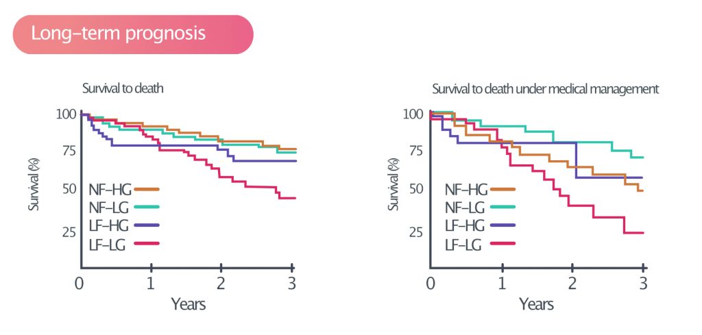
The aortic valve area is normally 3.0 to 4.0 cm2. Aortic stenosis is a progressive disease that leads to a gradual reduction in the orifice area. As the area is reduced, transvalvular flow resistance increases. This results in increased left ventricular load, while simultaneously affecting systemic perfusion. Aortic stenosis is a serious condition with poor long-term outcomes. Patients with low-flow low-gradient aortic stenosis (discussed below) have a 3-year survival rate of 50% (Eleid et al).
The cause of aortic stenosis displays marked geographical variations. In high-income countries, the majority of cases are caused by calcification of the aortic valve. Calcification has traditionally been considered a passive degenerative process, but emerging evidence suggests it is propelled by a biologically active process. Risk factors for calcification overlap with risk factors for coronary heart disease (atherosclerosis). The average age at diagnosis of aortic stenosis is 75 years in high-income countries.
In low- and middle-income countries, rheumatic heart disease is the leading cause of aortic stenosis. Rheumatic heart disease is a complication of rheumatic fever, which is caused by streptococcal infections (group A Streptococcus). Rheumatic heart disease can occur at any age and multiple valve lesions are common (typically the aortic and mitral valve). Rheumatic heart disease is rare in high-income countries, presumably because streptococcal infections are treated very liberally.
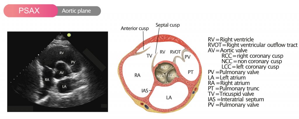
Figure 1 shows the aortic valve in PSAX (parasternal short-axis view).
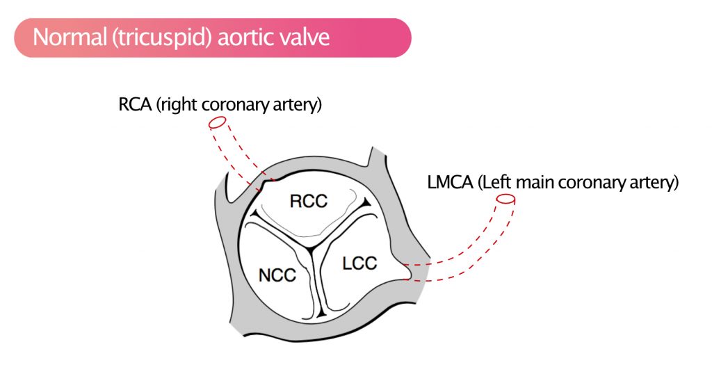
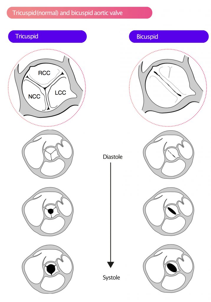
Individuals with bicuspid aortic valves have substantially elevated risk of developing aortic stenosis. The prevalence of bicuspid aortic valves is 1% to 2% in most Western populations. Individuals with bicuspid aortic valves may develop symptomatic aortic stenosis already at the age of 60 years. Bicuspid aortic valves also increase the risk of aortic aneurysm, aortic dissection, and endocarditis. Figure 2 shows the normal tricuspid aortic valve.
Natural course and prognosis in aortic stenosis
Aortic stenosis is generally asymptomatic until the valve area is <1 cm². This condition causes hemodynamic changes that alter ventricular volume load, myocardial wall stress and coronary artery perfusion. These changes gradually lead to insufficient coronary perfusion (i.e myocardial ischemia and angina pectoris), ventricular dysfunction (heart failure) and arrhythmias. The annual risk of sudden cardiac arrest is <1% and median survival is 3 years. Long-term prognosis in aortiv stenosis is presented in Figure 3.
Pathophysiology of aortic stenosis
As aortic stenosis progresses, pressure conditions on the left side change dramatically, including in the left ventricle, left atrium, aorta and coronary arteries.
As the valve area becomes smaller, the transvalvular resistance increases, making it more difficult to eject blood into the aorta. In the early stages of aortic stenosis, stroke volume becomes smaller. Reduced stroke volumes and increased resistance in the valve result in compensatory left ventricular hypertrophy. This allows the left ventricle to generate greater pressure, thereby overcoming the resistance in the stenosis and maintaining adequate stroke volumes.
Thus, ventricular hypertrophy is a compensatory mechanism, the purpose of which is to maintain sufficient stroke volumes. As discussed previously, afterload is the resistance that the muscle fibers must overcome to eject blood into the aorta; this is equivalent to the force that the myocardium must generate during systole. Afterload is described in terms of wall tension (wall stress), which is the load on individual muscle fibers. Wall stress per surface area (σ) can be calculated with Laplace’s law:
Wall stress = σ = (pLV × rLV) / (2 × thicknessLV)
LV = left ventricle; p = transmural pressure; r = radius,
This formula provides a mathematical explanation as to why aortic stenosis leads to hypertrophy. Aortic stenosis causes increased wall stress (i.e load on individual muscle fibers), which can be alleviated if the numerator becomes smaller or if the denominator becomes larger. In the early stages of aortic stenosis, wall thickness increases (i.e the denominator becomes larger), which results in a reduction in wall stress.
Unfortunately, left ventricular hypertrophy leads to cardiac remodeling, which in turn leads to reduced myocardial compliance. This is due to increased wall thickness and the development of interstitial fibrosis. As compliance decreases, passive filling of the left ventricle is reduced. Atrial contraction (active filling) becomes increasingly important. Impaired passive filling leads to higher end-diastolic pressure in the ventricle. It is believed that this results in reduced myocardial perfusion pressure, consequently, subendocardial ischemia. Elevated end-diastolic pressure can also propagate backward to the left atrium and further to the pulmonary circulation. Therefore, individuals with aortic stenosis may develop pulmonary edema.
As the stenosis becomes more pronounced, the progression of hypertrophy and fibrosis accelerates. Ventricular compliance decreases and filling pressure increases. Subendocardial ischemia develops, which, along with hypertrophy and fibrosis, leads to an increase in the risk of ventricular arrhythmias. Furthermore, stroke volumes are reduced as contractile function diminishes. When the myocardium can no longer compensate by hypertrophy, the ventricle begins to dilate. Ventricular dilatation leads to a decrease in intraventricular pressure and, consequently, a decrease in wall stress. This second compensatory mechanism ultimately leads to heart failure.
Angina pectoris (chest pain) and arrhythmias caused by aortic stenosis
Angina pectoris is common in aortic stenosis. Ischemia is explained by a decrease in coronary perfusion (the stenosis prevents normal blood flow through the aorta) in parallel with increased oxygen demand in the hypertrophic myocardium.
Aortic stenosis (AS) can also cause syncope, especially during physical activity. The mechanisms explaining how physical activity leads to syncope remain incompletely understood. With regards to arrhythmias, acute heart failure and syncope, the following explanations have typically been proposed:
- Ventricular arrhythmias in aortic stenosis (AS) are provoked by physical activity.
- Acute heart failure in AS occurs due to sudden ventricular overload.
- Sudden peripheral vasodilatation during or immediately after physical activity may also cause syncope.
Echocardiographic assessment of aortic stenosis
The majority of all patients with aortic stenosis can be diagnosed and monitored with echocardiography. In selected cases, assessment and follow-up may be supplemented by cardiac catheterization, magnetic resonance imaging (cardiac MRI) or computed tomography (CT). The key parameters for assessing aortic stenosis are presented in Table 1. As evident in Table 1, aortic stenosis is graded from sclerosis to severe aortic stenosis.
Table 1. Aortic stenosis grades of severity
| Echo parameter | Aortic valve sclerosis | Mild AS | Moderate AS | Severe AS |
|---|---|---|---|---|
| Peak velocity, m/sec | <2.5 | 2.5-3 | 3-4 | >4 |
| Mean gradient, mmHg | Normal | <20 | 20-40 | 40 |
| Aortic valve area, cm² | Normal | ≥1.5 | 1-1.5 | <1 cm² |
| Calcium scoring, AU* | Male: 2,065 Female: 1,275 |
*Calcium scoring obtained with computed tomography (CT).
Visual (2D) assessment of the aortic valve
Bicuspid aortic valves
In 80% of cases with bicuspid aortic valves, the RCC and LCC are fused, and in remaining cases, the RCC and NCC are fused. A normal (tricuspid) aortic valve has three cusps, which is most often evident in the parasternal short-axis (PSAX) view. During systole, the valve orifice is circular (Figure 4). A bicuspid aortic valve, on the other hand, has two cusps, which are usually asymmetric and differ in size. Occasionally, bicuspid valves may exhibit a clear raphe, which results in a tricuspid appearance of the valve on echocardiogram. A bicuspid aortic valve displays an elliptical orifice during systole (Figure 4).
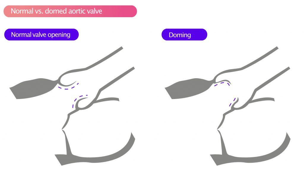
During systole, the cusps often display doming, as illustrated in Figure 5.
Calcification of the aortic valve
Calcification of the aortic valve appears as deposits with high echogenicity. Calcifications may be seen on the cusps, aortic annulus and proximal aorta. The extent and severity of valvular calcification can be graded semiquantitatively as mild (presence of small hyperechogenic areas with little acoustic shadowing), moderate (multiple large areas with dense echogenicity), or severe (extensive thickening with increased echogenicity and high acoustic shadowing).
Rheumatic heart disease
Aortic stenosis as a result of rheumatic heart disease results in a homogeneous thickening of the cusps, especially at the tips. In pronounced cases, the cusps may be fused at the tips. The cusps often display doming during systole (Figure 4).
Subvalvular obstruction
Subaortic obstruction implies that the stenosis is located in the LVOT (left ventricular outflow tract). Subvalvular stenosis is typically due to the presence of a subaortic membrane or HOCM (hypertrophic obstructive cardiomyopathy).
Subaortic membrane
A subaortic membrane is best visualized in apical views (4C, 5C) and appears as a distinct fibrous ring proximal to the aortic valve. The existence of a subaortic membrane causes turbulence in the LVOT. This can lead to incomplete valve closure during diastole, which in turn may lead to aortic regurgitation.
In HOCM, there are two factors contributing to the narrowing of the LVOT:
- Hypertrophy of the septum leads to narrowing of the LVOT.
- SAM (Systolic Anterior Motion) implies that the anterior mitral leaflet is pulled into the LVOT during systole, thereby obstructing the LVOT.
Supravalvular obstruction
Obstruction in the proximal aorta is a rare congenital malformation. It is typically visualized in PLAX (parasternal long-axis view).
Two-dimensional (2D) echocardiography
LVOT and proximal aorta
The following measurements, illustrated in Figure 6, should be performed:
- LVOT (left ventricular outflow tract)
- Aortic annulus
- Sinus of Valsalva
- Sinotubular junction (STJ)
- Ascending aorta
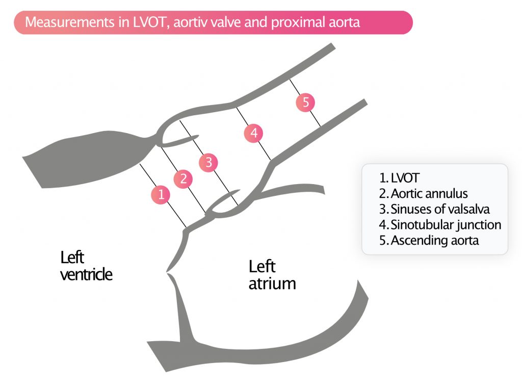
Measurements are made when the valve is open (i.e during systole). Dilatation of the aortic annulus, sinus of Valsalva, STJ (sinotubular junction) and ascending aorta should lead to suspicion of Marfan syndrome or bicuspid aortic valves, especially among younger individuals. Dilatation is also seen in systemic hypertension and in older individuals.
Evaluation of the left ventricle
The left ventricle should be investigated in terms of hypertrophy and dilatation. Refer to Left Ventricular Size and Dimensions.
Doppler studies
Doppler examination provides the most objective quantification of the severity of aortic stenosis. It is of prime importance to record the peak flow velocity, using continuous Doppler, across the aortic valve. The peak velocity is used to calculate the pressure gradient (i.e pressure difference) across the aortic valve. The more severe the stenosis, the greater the pressure gradient and, accordingly, the velocity across the valve. Measurements are always performed in multiple apical views, and mostly also from right-sided parasternal view and suprasternal view.
A pencil probe (PEDOF [Pulse Echo DOppler Flow] probe) may be necessary to capture high velocities (>3.5 m/s) with precision. The pencil probe is a small dual-crystal continuous wave transducer, which allows for optimal transducer positioning, angulation, and measurement of high velocities. The pencil probe may be used in any view, particularly right parasternal and suprasternal views. However, it is generally not necessary if flow velocity is low (<3 m/s) and cusp opening can be visualized clearly. The disadvantage of the pencil probe is the lack of a 2D image to guide the ultrasound.
Peak gradient across the aortic valve
The maximum (peak) gradient represents the greatest pressure difference recorded across the valve during systole. This is obtained by recording the peak velocity (using continuous Doppler) across the valve during systole. The peak velocity is entered into Bernoulli’s simplified formula to calculate the peak gradient (ΔP, mmHg):
ΔP = 4v2
Mean gradient across the aortic valve
The mean gradient represents the mean pressure difference between the left ventricle and the aorta during systole. This is calculated by using continuous Doppler to obtain VTI (Velocity Time Integral) across the valve. If the mean gradient across the aortic valve is ≥40 mmHg, then the aortic stenosis is graded as severe.
Aortic valve area (AVA)
The opening area of the aortic valve is calculated using the continuity equation. The underlying principle is that the volume of blood that flows (per unit time) through the aortic valve must be equal to the volume flowing through LVOT. Recall that VTI and area can be used to calculate volume: volume = area × VTI. According to the continuity equation, the product of area and VTI must be equal in the LVOT and aortic valve:
areaLVOT × VTILVOT = areaaortic valve × VTIaortic valve
To calculate aortic valve area, we measure areaLVOT, VTILVOT and VTIaortic valve. The areaLVOT is obtained by measuring the diameter (D) of LVOT:
areaLVOT = DLVOT × π
VTILVOT is calculated using pulsed wave Doppler with sample volume placed in LVOT. VTIaortic valve is measured with continuous wave Doppler through the aortic valve. Then areaaortiv valve is calculated as follows:
areaaortic valve = (areaLVOT × VTILVOT)/VTIaortic valve
The aortic valve area can be adjusted for body surface area (BSA). If the aortic valve area is <1 cm2 or BSA normalized area is <0.6 cm2/m2, then the aortic stenosis is severe.
If the velocity in LVOT is >1.5 m/s or if the velocity across the aortic valve is <3.0 m/s, the pressure gradient should be calculated using the following formula:
ΔP = 4(v2aortiv valve – v2LVOT)
VTI ratio
VTI ratio can also be used to estimate the degree of stenosis.
VTILVOT / VTIaortic valve
The lower the ratio, the more pronounced the stenosis. VTI ratio <0.25 implies severe aortic stenosis. VTI ratio is especially useful in individuals with small ventricular volumes.
In the setting of atrial fibrillation, all measurements should be made on 5 consecutive cardiac cycles and the mean value of each respective parameter should be used to perform the calculations.
Pressure recovery phenomenon: overestimation of the pressure gradient
According to Bernoulli’s law, pressure drops and velocity increases as a liquid travels towards a narrowing. Once the liquid has passed the narrowing, the opposite occurs; velocity decreases and pressure increases. This also applies to blood flow through stenotic valves. The phenomenon is called pressure recovery phenomenon (Figure 7).
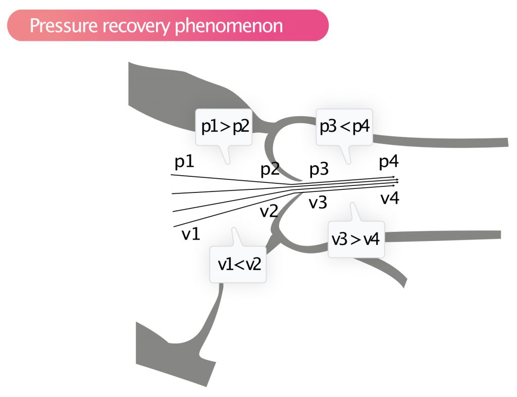
Pressure recovery implies that the pressure increases rapidly immediately after a stenosis, while velocity diminishes. With continuous wave Doppler, the highest velocity is recorded, which is the velocity immediately after stenosis and where the pressure is actually lower than the pressure further up in the aorta. Thus, Doppler will overestimate the pressure drop across the aortic valve; i.e, the difference between the pressure in the aorta and the left ventricle is lower than what the Doppler measurement suggests. The smaller the aortic diameter, the more pronounced the pressure recovery. If the ascending aorta is <3.0 cm, then, generally, there is significant pressure recovery in aortic stenosis. If the ascending aorta is wide, then pressure recovery can be ignored.
Classification of aortic stenosis
Patients with an aortic valve area <1 cm² (and preserved ejection fraction) can be classified into four groups according to mean pressure gradient (MPG) and stroke volume index (SVI). The latter is the stroke volume normalized to body surface area (BSA).
| High flow / High gradient | MPG >40 mmHg SVI ≥35 ml/m² |
| High flow / Low gradient | MPG <40 mmHg SVI ≥35 ml/m² |
| Low flow / High gradient | MPG >40 mmHg SVI <35 ml/m² |
| Low flow / Low gradient | MPG <40 mmHg SVI <35 ml/m² |
Low flow, low gradient, low EF aortic stenosis
The pressure gradient is fundamental in aortic stenosis. In the setting of contractile (systolic) dysfunction, the left ventricle is unable to generate a normal increase in pressure and, accordingly, the pressure gradient across the aortic valve decreases, regardless of the stenosis. Hence, a patient with aortic stenosis who develops contractile dysfunction will display improvement in the pressure gradient, despite the fact that the stenosis remains unchanged, or even more severe.
This scenario is referred to as low flow, low gradient, low ejection fraction aortic stenosis. On echocardiography, this is characterized by the following:
- Aortic valve area <1 cm2
- LVEF (ejection fraction) <40%
- Mean pressure gradient <30–40 mmHg.
Furthermore, contractile dysfunction may lead to the aortic valve appearing less mobile than it actually is. This is explained by the fact that the dysfunctioning ventricle is unable to generate enough force to open the valves properly (particularly if they are calcified). In this scenario, moderate aortic stenosis may appear as severe. This is referred to as pseudosevere aortic stenosis. In such cases, it is especially important to calculate the aortic valve area.
Low flow, low gradient, normal EF aortic stenosis
Individuals with small ventricular volumes may exhibit low flow, low gradient, normal EF aortic stenosis, which implies that aortic stenosis is present with low flow and low gradient despite normal ejection fraction. In these situations, the VTI ratio should be given greater importance in the assessment.
Echocardiographic assessment of the severity of aortic valve stenosis relies on peak velocity, mean pressure gradient and aortic valve area (AVA), which should ideally be concordant. In 25% of patients these parameters are discordant (usually aortic valve area <1 cm² and mean pressure gradient <40 mmHg). In most cases, these patients present with a normal flow (stroke volume index ≥35/ml/m²) but low flow provides important prognostic information. To assess whether these patients truly present with severe aortiv stenosis, calcium score should be measured using computed tomography (thresholds are 2,000 AU in male and 1,250 AU in female) [1].
References
[1] Messika-Zeitoun et al. Aortic valve stenosis: evaluation and management of patients with discordant grading.
[2] Baumgartner et al. Recommendations on the Echocardiographic Assessment of Aortic Valve Stenosis: A Focused Update From the European Association of Cardiovascular Imaging and the American Society of Echocardiography.