Strain, strain rate and speckle tracking: Myocardial deformation
Myocardial deformation: strain, strain rate, speckle tracking
As previously discussed, the left ventricular wall can be subdivided into three layers: the inner lining (endocardium), a thick muscle layer (myocardium) and an outer lining (epicardium). The myocardium is the thick muscle layer, in which the muscle fibers are organized into several sheets wrapping around the ventricle with varying orientation. This organization allows the left ventricle to contract in a highly sophisticated and effective way (Figure 1).
Myocardial fibers adjacent to the endocardium are longitudinally oriented (from base to apex) and yield a longitudinal shortening (Figure 1A), which means that the base is pulled towards the apex.
Myocardial fibers in the middle layer (mid-wall) are oriented circularly around the short-axis. Contraction in this layer results in radial shortening, meaning that the diameter of the ventricular cavity decreases (Figure 1B).
The muscle fibers adjacent to the epicardium are oriented approximately 60° in relation to the fibers of the mid-wall. Contraction in this layer results in a twisting (rotating) motion of the entire left ventricle. Basal segments rotate clockwise, and the apex rotates counterclockwise. This rotating, or twisting, contraction is called circumferential shortening (Figure 1C).
Left ventricular function depends on a complex interaction between the muscle fibers in these layers, which collectively produces a highly efficient pumping mechanism.
Traditional methods for investigating left ventricular function — e.g ejection fraction (EF), fractional sorting (FS), etc — do not elucidate regional variations in contractile function, or the effectiveness of longitudinal, radial, and circumferential contraction. Thus, methods such as ejection fraction may provide easily obtained parameters, but fail to provide important insights into left ventricular mechanics.
Regional differences in contractile function are of utmost importance, particularly in the setting of (confirmed or suspected) myocardial ischemia. As a clear example, consider a patient with ischemic heart disease, who has normal ejection fraction but impaired contractile function in the inferior wall. This finding is referred to as inferior wall motion abnormality and it may evidence of myocardial infarction, which would have implications for the management of this patient, regardless of the ejection fraction. Hence, it is important to detect and characterize wall motion abnormalities.
Methods have been developed for the quantification of regional myocardial function. These methods analyze the motion and deformation (change in shape) of the myocardium during systole and diastole. Deformation imaging has been implemented in clinical practice and is now widely recommended. This chapter discusses the theoretical and practical aspects of deformation (strain, strain rate) and myocardial motion.
Myocardial motion
Myocardial motion concerns the movement of myocardium from one point to another. During the motion, all myocardium within a particular region displays the same velocity. The motion is characterized by two variables: distance and velocity. Distance denotes the distance the myocardium travels, and velocity denotes the speed of the motion.
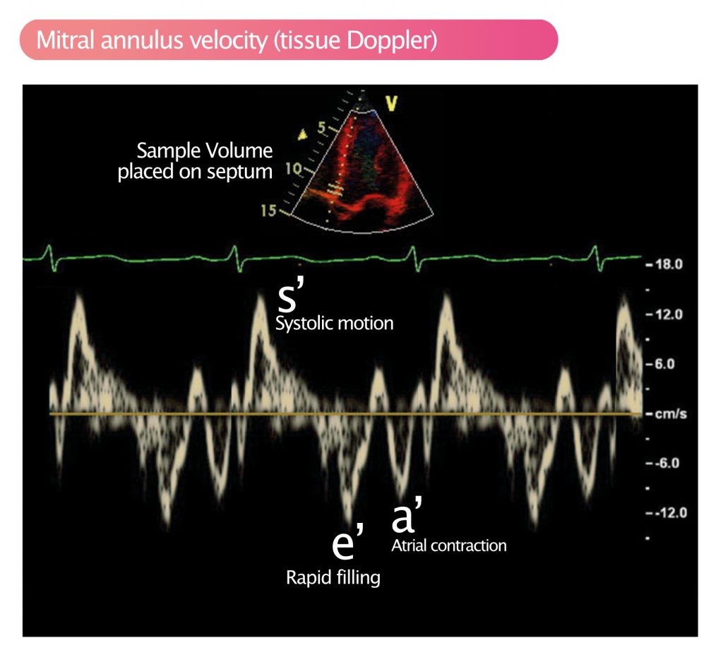
Myocardial motion and velocity can be measured with pulsed tissue Doppler (see Pulsed Wave Doppler). Tissue Doppler allows for sampling of specific regions or structures. This is done by placing the sample volume (SV) in the region of interest. This is routinely done to measure the velocity of the mitral annulus, which during systole travels towards the apex, and then recoils to its starting position. Mitral annulus velocity is used to study longitudinal contraction; during systole, the base, and thus the mitral annulus, moves towards the apex and during diastole, the opposite motion occurs. The mitral annulus velocity is an important measure of global longitudinal systolic function. Figure 2 demonstrates the measurement of mitral annulus velocity with pulsed tissue Doppler.
Color tissue Doppler can also be used to study regional velocities. It has the advantage of studying larger areas of myocardium simultaneously, which does, however, come at the expense of lower temporal resolution.
Disadvantages of using motion as a marker of function
The major disadvantage of using motion as a measure of regional contractile function is that all myocardium is interconnected. Motion in one area is directly affected by motion in adjacent areas. This allows even necrotic myocardium (e.g due to myocardial infarction) to move during systole and diastole (viable and contracting myocardium surrounding the necrotic zone will pull and push the dead myocardium, such that it displays a motion). It follows that measurement of motion in a single point can be highly misleading since the motion in one point depends on the motions of the surrounding myocardium.
The solution is to use deformation as a measure of function. The rationale for measuring deformation is that dead myocardium will not deform (change shape) during systole and diastole, regardless of motions in surrounding myocardium. Measuring deformation has proven to be superior to measuring motion.
Strain and strain rate: Measures of deformation
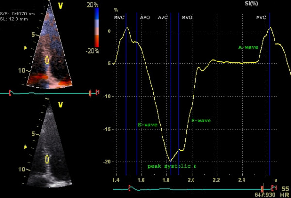
Strain is defined as shortening or lengthening of myocardium. Shortening occurs when myocardium contracts, and lengthening occurs when myocardium relaxes (stretches out). These two deformations can be studied by means of echocardiography. The main objective is to determine whether myocardial motion is normal by measuring the degree of deformation (strain) and the speed at which it occurs (strain rate).
Strain and strain rate should be relatively similar throughout the myocardium since all regions should deform approximately equally during the cardiac cycle. Examination of strain and strain rate can identify regional differences in deformation, which indicates pathology. Moreover, it can elucidate the overall myocardial deformation, which is an indicator o global function.
Strain: The degree of deformation
Strain is the degree of deformation, i.e. how much the myocardium is deformed. It is calculated by measuring the extent of shortening or lengthening during the cardiac cycle. The formula for strain is as follows:
Strain = (L–L0)/L0·100
L0 = initial myocardial length; L = final length.
The constant 100 transforms strain into percent (%).
If the initial length of the area measured is 10 mm and the final length is 12 mm, then strain will be +20% (positive strain). If the initial length is 10 mm and the final length is 7 mm, then strain will be –30% (negative strain). Contraction (shortening) gives negative strain and relaxation (lengthening) gives positive strain (Figure 3).
Strain can be measured in all directions of deformation; it is possible to study longitudinal, radial and circumferential strain.
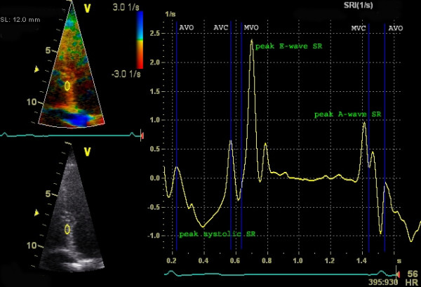
Strain rate: the speed of deformation
Strain rate is the speed of deformation, i.e. deformation per unit time (seconds). It can be mathematically proven that deformation per unit time is equivalent to the difference in velocity within an area divided by the length of the area, as follows:
Strain rate = (V1 – V2) / d
According to the above formula, strain rate can be obtained by measuring the velocity (using pulsed tissue Doppler) in two points of myocardium, and the distance between the points (Figure 4).
Strain rate is a measure of the velocity of deformation between two measurement points. As for strain, a negative value indicates contraction, and a positive value indicates relaxation.
By mapping strain rate in many parts of the myocardium simultaneously, it is possible to determine if strain and strain rate is equal in all parts, which is expected. Pulsed tissue Doppler computes both strain and strain rate simultaneously.
To calculate strain and strain rate using tissue Doppler, a frame rate of 100 FPS is used. The advantage of tissue Doppler is that the temporal resolution is very high and the method is adequate for measuring longitudinal strain. Unfortunately, tissue Doppler is angle dependent (incorrect angle of insonation leads to an underestimation of strain rate) and, moreover, radial and circumferential strain cannot be investigated. These shortcomings have been overcome by means of speckle tracking, which is discussed next.
Speckle tracking
Speckle is the term for the structures that the myocardium displays on the ultrasound image. If you carefully examine Figure 7, you can see that the myocardium does not produce a homogeneous signal, but a pattern of variations in the echo signal is seen. These structures are called speckles and they arise due to the interactions of ultrasonic waves (reflections, proliferation, interference) with the tissue.
Speckle tracking
Speckles move during systole and diastole and it is possible to analyze the velocity and distance of their motions. This is called speckle tracking and this method has largely replaced tissue Doppler to measure strain and strain rate. Figure 9 illustrates how speckles are tracked in the two-dimensional plane. Strain is defined as the change in the distance between two speckle-points, divided by the initial distance:
S = (L1−L0) / L0
L0 = initial distance between the points.
L1 = new distance between the points.
Speckle tracking is entirely based on the ultrasound image, and no Doppler measurements are required. This makes speckle tracking more reliable since it is not sensitive to the angle of insonation. However, speckle tracking offers a lower temporal resolution, which makes the method poorer in the setting of tachycardia (precision is reduced at high heart rate) and when studying speckles located remotely (from the transducer). Moreover, speckle tracking is inferior for lateral motions, which is due to the fact that ultrasound has a lower lateral resolution, as compared with axial resolution.
Speckle tracking uses 40 to 80 FPS (frames per second) and up to 100 FPS may be needed during tachycardia. Speckle tracking can be used for all four chambers, although measurements in the right atrium and right ventricle are generally less precise due to difficulties identifying speckles.
Global and regional strain
Modern ultrasound systems calculate both regional and global strain. Regional strain is the strain calculated in each segment. Global strain is the average of all individual segments.
With speckle tracking, strain and strain rate can be calculated for movements in longitudinal, radial and circumferential directions. In apical four-chamber view (A4C), the longitudinal strain is most important. Longitudinal strain is a robust marker of cardiac function and correlates well with, for example, ejection fraction (EF). The longitudinal deformation depends primarily on subendocardial muscle fibers since these are oriented in the longitudinal direction. Circumferential deformation (best analyzed in PSAX) primarily reflects epicardial fibers. Longitudinal strain decreases in diseases such as hypertension, diabetes, and cardiomyopathy.